Technical Details

This section will go into detail about each back-end implementation, as well as the blue noise variants. Here you can find out about practical trade-offs for each option, so you can decide which is best for your use case.

PMJ sequences

The implementation uses the stochastic method described by Helmer et la. [^2] to efficiently construct a progressive multi-jittered (0,2) sequence. The first pair of dimensions in a domain have the same integration properties as the Sobol implementation. However, as the sequence doesn't extend to more than two dimensions, the second pair is randomised relative to the first in a single domain.

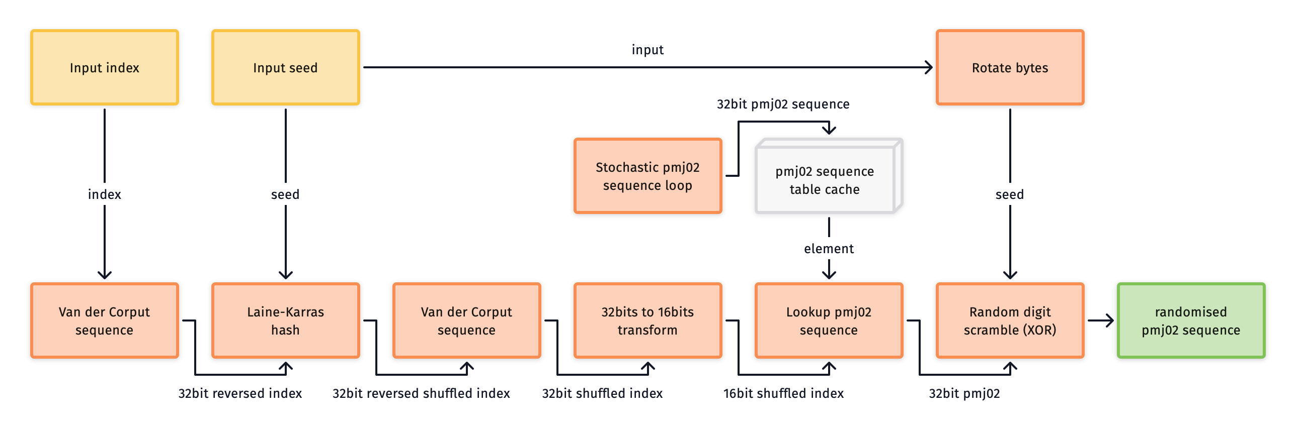
This sampler pre-computes a base 4D pattern for all sample indices during the cache initialisation. Permuted index values are then looked up from memory at runtime, before being XOR scrambled. This amortises the cost of initialisation. The rate of integration is very high, especially for the first and second pairs of dimensions. You may however not want to use this implementation if memory space or access is a concern.

Sobol sequences

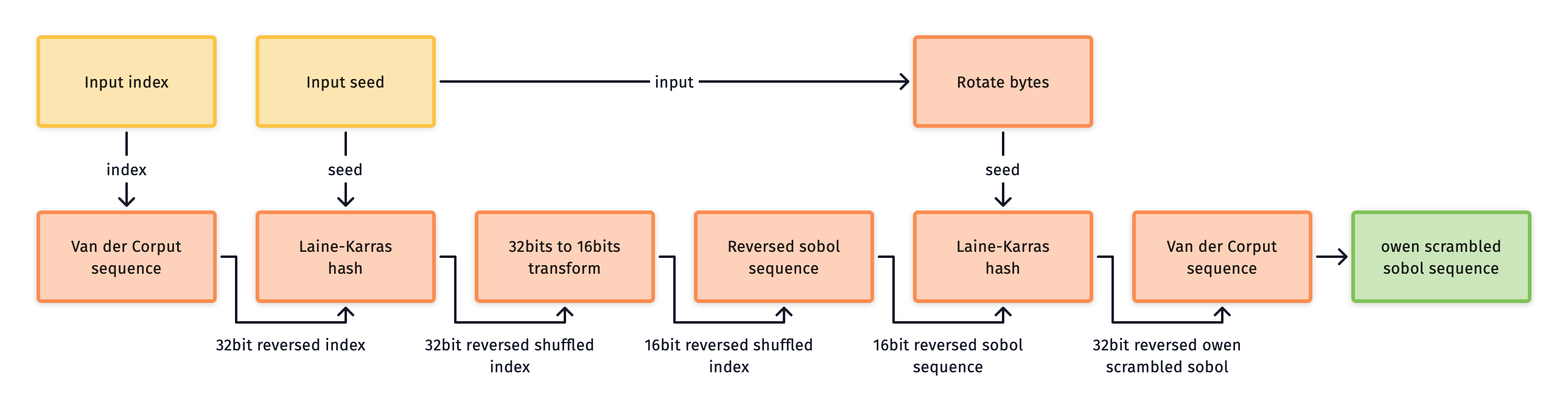
The implementation uses an elegant construction by Burley [^1] for an Owen scrambled Sobol sequence. This also includes performance improvements such as limiting the index to 16 bits, pre-inverting the input and output matrices, and making use of CPU vector intrinsics. You need to select a OPENQMC_ARCH_TYPE to make use of the performance from vector intrinsics for a given architecture.

This sampler has no cache initialisation cost, it generates all samples on the fly without touching memory. However, the cost per draw sample call is computationally higher than other samplers. The quality of Owen scramble sequences often outweigh this cost due to their random error cancellation and incredibly high rate of integration for smooth functions.

Lattice sequences

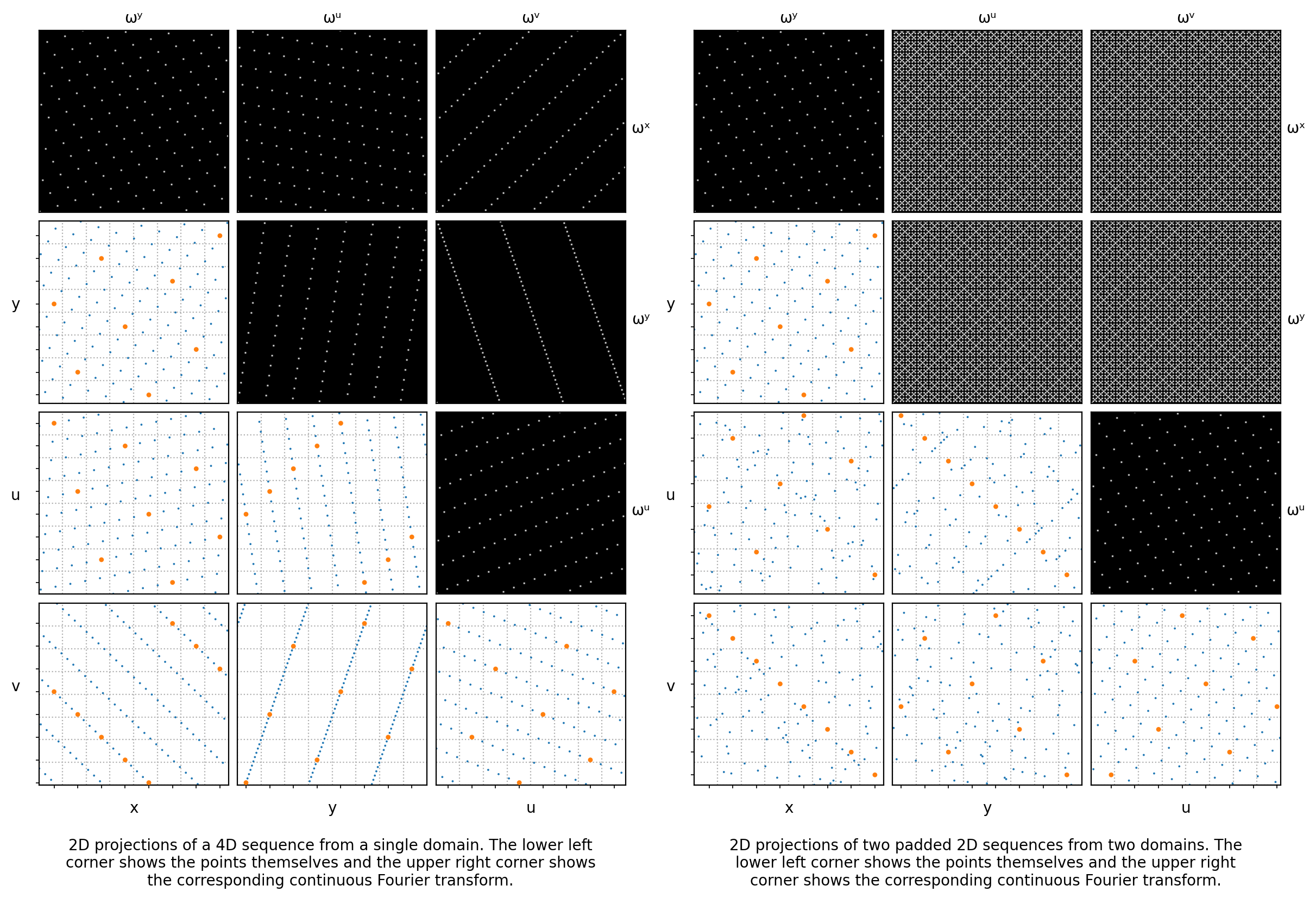
The implementation uses the generator vector from Hickernell et al. [^3] to construct a 4D lattice. This is then made into a progressive sequence using a scalar based on a radical inversion of the sample index. Randomisation uses toroidal shifts.

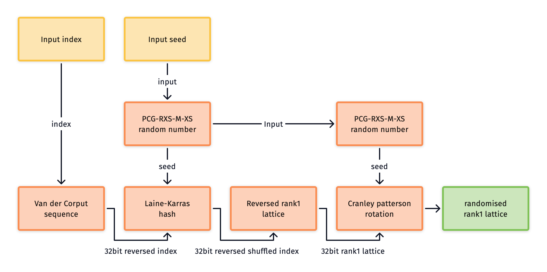
This sampler has no cache initialisation cost, it generates all samples on the fly without touching memory. Runtime performance is also high with a relatively low computation cost for a single draw sample call. However, the rate of integration per pixel can be lower when compared to other samplers.

Blue noise sampler variants

Blue noise variants offer spatial blue noise dithering between pixels, with progressive pixel sampling. This is done using an offline optimisation process that's based on the work by Belcour and Heitz [^4].

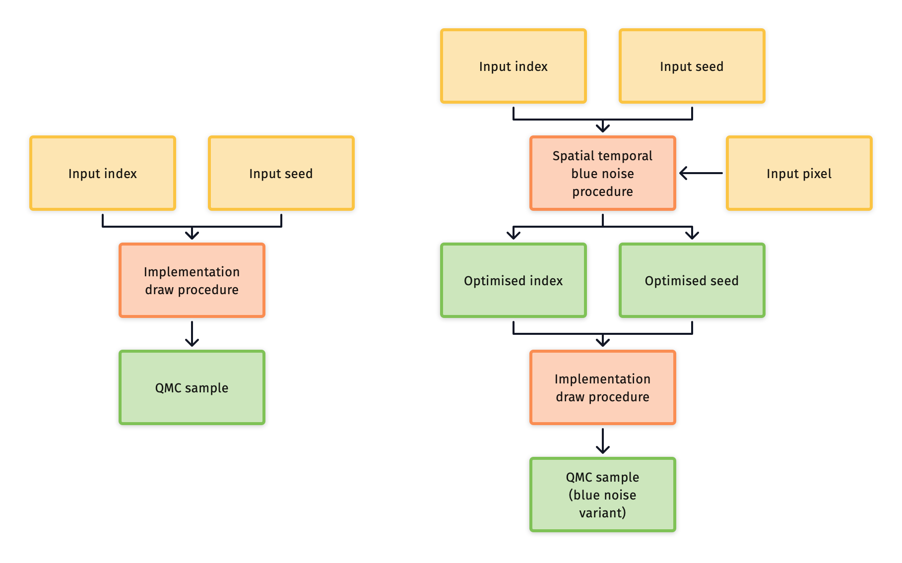
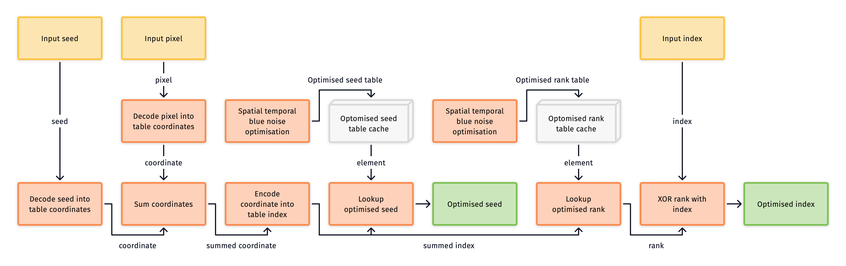
Each variant achieves a blue noise distribution using two pixel tables, one holds keys to seed the sequence, and the other index ranks. These tables are then randomised by toroidally shifting the table lookups for each domain using random offsets. Correlation between the offsets and the pixels allows for a single pair of tables to provide keys and ranks for all domains.

Although the spatial blue noise doesn't reduce the error for an individual pixel, it does give a better perceptual result due to less low frequency structure in the error between pixels. Also, if an image is either spatially filtered (as with denoising), the resulting error can be much lower when using a blue noise variant as shown in Rate of convergence.

Blue noise variants are recommended, as the additional performance cost will likely be a favourable tradeoff for the quality gains at low sample counts. However, access to the data tables can impact performance depending on the architecture (e.g. GPU), so it is worth benchmarking if this is a concern.

For more details, see the Optimise CLI in the Tools section.

Passing and packing samplers

Sampler objects can be efficiently passed by value into functions, as well as packed and queued for deferred evaluation. Achieving this means that the memory footprint of a sampler must be very small, and the type trivially copyable.

Sampler types are either 8 or 16 bytes in size depending on the type. The small memory footprint is possible due to the state size of PCG-RXS-M-RX-32 from the PCG family of PRNGs as described by O'Neill [^6].

When deriving domains the sampler will use an LCG state transition, and only perform a permutation prior to drawing samples analogous to PCG. This provides high quality bits when drawing samples, but keeps the cost low when deriving domains, which might not be used.