Increasing Sampling Rate

Domain splitting

Whereas domain branching lets you sample different dimensions within each sample index, domain splitting is an operation to sample given dimensions with a higher sampling rate. Splitting allows you to tackle high variance in specific dimensions without the cost for the increased sampling rate on all dimensions.

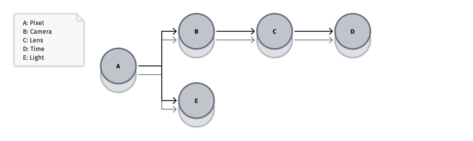
The diagram above shows the same domain tree extended with a stack for each domain. Each stack element represents an index in the domain's pattern. This example begins with two indices for each domain.

If you were to consider direct light sampling, which is often a source of high variance. One possible approach is to sample lights at a higher rate than pixels by defining a multiplier on that rate, such as N_LIGHT_SAMPLES.

Result estimatePixel(const oqmc::PmjBnSampler pixelDomain,
                     const CameraInterface& camera,
                     const LightInterface& light)
{
    enum DomainKey
    {
        Camera,
        Light,
    };

    // Compute 'cameraSample' as in previous examples.
    const auto cameraDomain = pixelDomain.newDomain(DomainKey::Camera);
    const auto cameraSample = camera.sample(cameraDomain);

    auto result = Result{};

    // Loop a fixed N times.
    for(int i = 0; i < N_LIGHT_SAMPLES; ++i)
    {
        // Compute 'lightSample' using the newDomainSplit API.
        const auto lightDomain = pixelDomain.newDomainSplit(DomainKey::Light, N_LIGHT_SAMPLES, i);
        const auto lightSample = light.sample(lightDomain);

        // Average the pixel estimates from each light sample.
        result += estimateLightTransport(cameraSample, lightSample) / N_LIGHT_SAMPLES;
    }

    return result;
}

Here the calling code derives a lightDomain in a loop, using a different function than the other examples. Along with a key, this new function takes a fixed sample rate multiplier and an index within the multiplier range. You must pass all indices to the API and average the results.

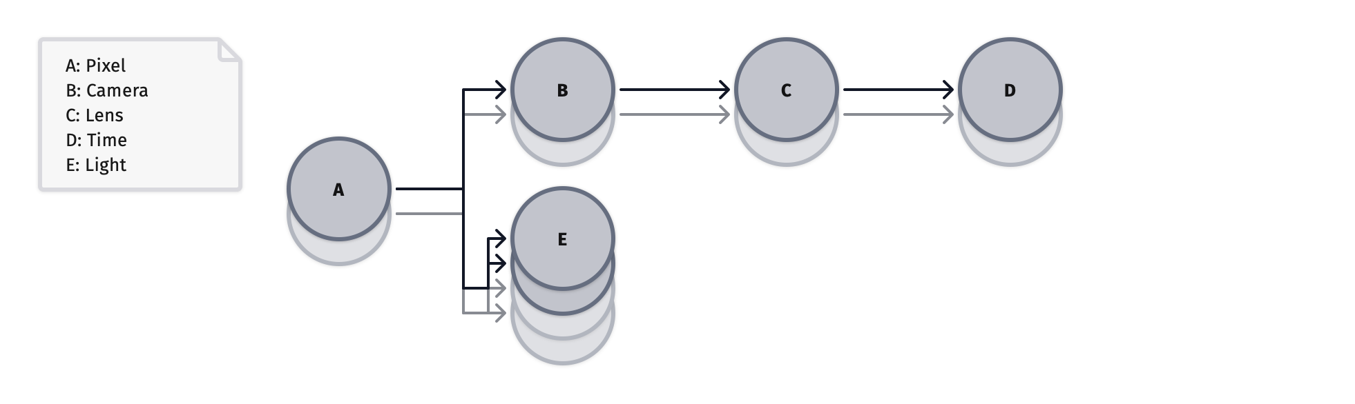
In this domain tree, N_LIGHT_SAMPLES maintains a fixed value of 2, and thus, the light domain's sampling rate is twice that of the source pixel domain.

A fixed sample rate multiplier like the one in this example correlates points globally and locally. This correlation makes the pattern optimal while saving compute costs in other domains. The following section will give options for when the sample rate multiplier is non-constant.

Adaptive rate multipliers

Sometimes, the constraint of a fixed sample rate multiplier is not an option or is undesirable. In these cases, a couple of alternative strategies trade quality for the added flexibility of non-constant multipliers.

Result estimatePixel(const oqmc::PmjBnSampler pixelDomain,
                     const CameraInterface& camera,
                     const LightInterface& light)
{
    enum DomainKey
    {
        Camera,
        Light,
    };

    // Compute 'cameraSample' as in previous examples.
    const auto cameraDomain = pixelDomain.newDomain(DomainKey::Camera);
    const auto cameraSample = camera.sample(cameraDomain);

    // Compute a non-fixed number of light samples.
    const auto nLightSamples = light.adaptiveSampleRate();

    auto result = Result{};

    // Loop a non-fixed N times.
    for(int i = 0; i < nLightSamples; ++i)
    {
        // Compute 'lightSample' using the newDomainDistrib API.
        const auto lightDomain = pixelDomain.newDomainDistrib(DomainKey::Light, i);
        const auto lightSample = light.sample(lightDomain);

        // Average the pixel estimates from each light sample.
        result += estimateLightTransport(cameraSample, lightSample) / nLightSamples;
    }

    return result;
}

This example has a non-constant sample rate multiplier nLightSample for the light domain. Here, the caller uses the alternative newDomainDistrib function that allows for varying sample rate multipliers. Using this technique is called the distribution strategy.

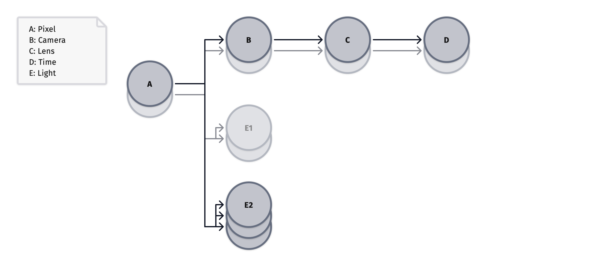
Here is the domain tree when using the distribution strategy. The split domain is not correlated globally, but it is locally. The domain is in fact branched into two locally correlated domains, one for each index from the source pixel domain. The first has a sample rate of 2, and the second a sample rate of 3, based on nLightSamples.

Result estimatePixel(const oqmc::PmjBnSampler pixelDomain,
                     const CameraInterface& camera,
                     const LightInterface& light)
{
    enum DomainKey
    {
        Camera,
        Light,
    };

    // Compute 'cameraSample' as in previous examples.
    const auto cameraDomain = pixelDomain.newDomain(DomainKey::Camera);
    const auto cameraSample = camera.sample(cameraDomain);

    // Compute a non-fixed number of light samples.
    const auto nLightSamples = light.adaptiveSampleRate();

    auto result = Result{};

    // Loop a non-fixed N times.
    for(int i = 0; i < nLightSamples; ++i)
    {
        // Compute 'lightSample' by chaining the newDomain API.
        const auto lightDomain = pixelDomain.newDomainChain(DomainKey::Light, i);
        const auto lightSample = light.sample(lightDomain);

        // Average the pixel estimates from each light sample.
        result += estimateLightTransport(cameraSample, lightSample) / nLightSamples;
    }

    return result;
}

This last example is similar to the distribution strategy. But here the caller uses the newDomainChain function, which is the equivalent of chaining two newDomain functions. This technique is called the chaining strategy.

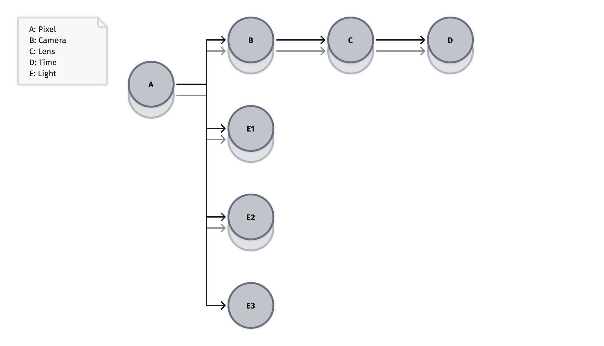
Here is the domain tree when using the chaining strategy. This new domain is correlated globally, but it is not locally. Each of the sample indices from the source pixel domain is free to branch at non-constant rate. The first branches into 2 domains, and the second into 3 domains, based on nLightSamples.

Notice that the transformation of the light domain tree between the distribution and the chaining strategies is a transposition. And the optimal choice between both of these strategies will depend on the ratio between the global and the local sample rate multipliers. In this example the distribution strategy is optimal because the local sample rate multiplier is higher than the global.

So which strategy to choose? Following are the results from each strategy. Numbers after each strategy indicate RMSE. As expected, the initial option of splitting using a fixed sample rate multiplier produces the best results.

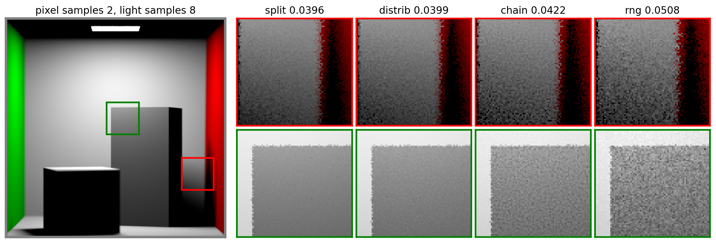
But when that isn't possible and using a non-constant sample rate multiplier, and that multiplier is expected to be higher than the source pixel sample rate, the distribution strategy is optimal as it is locally correlated.

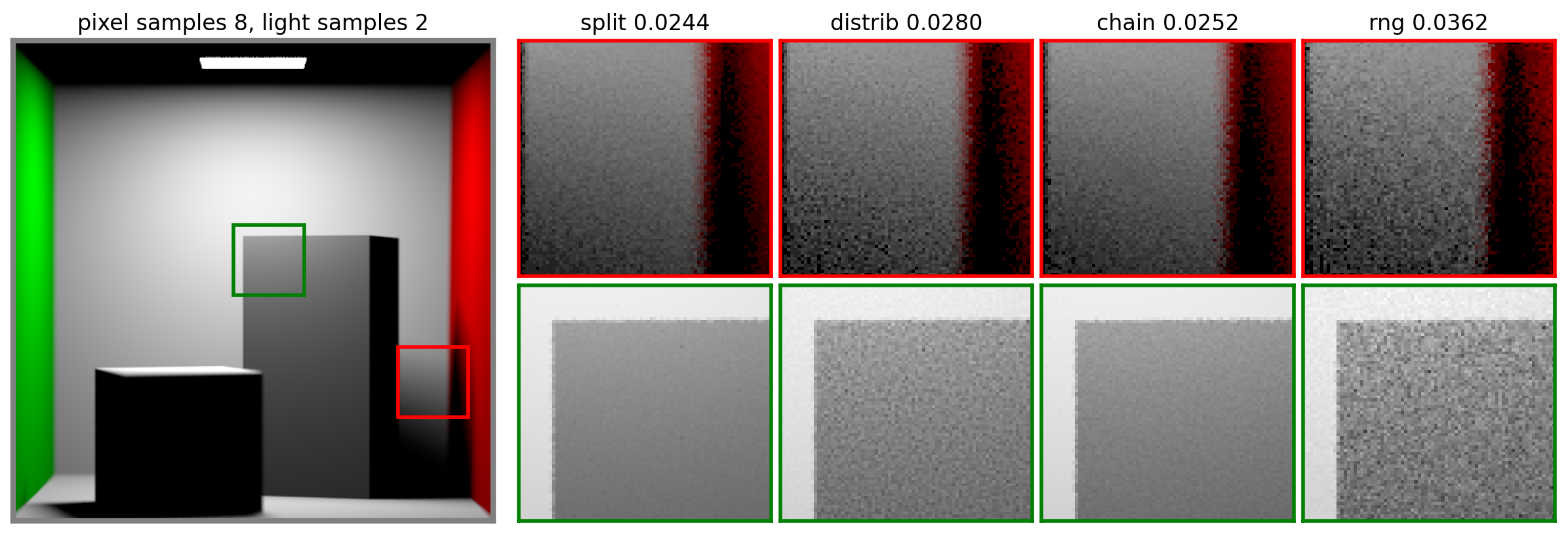
However, when an adaptive sample rate multiplier is expected to be lower than the original pixel sample rate, as demonstrated here, the chaining strategy is optimal as it is globally correlated.